The Genesis of the Quant – From Physics to Neural Networks

Understanding where quantitative development came from matters. To build a modern AI-driven trading system, you have to stand on 100 years of Random Walk theory. The 1980s were about closed-form formulas; the 2020s are about data and patterns.

In this post: How Brownian motion, Black-Scholes, and machine learning shaped quant dev—and why Python, TensorFlow, and LLMs define the future of algorithmic trading.

Key takeaways:

• 1827–1930: Brown → Bachelier → Einstein → Wiener → Ornstein-Uhlenbeck: the full arc of Brownian motion
• 1963–1990s: Mandelbrot’s fat tails, Black Monday’s volatility smile, ARCH/GARCH—where formulas broke
• Data-first shift: Quant dev moved from closed-form math to training models with Python and ML
• Stack roadmap: Pandas → visualization → Keras/TensorFlow → LangChain/LLMs

Figures in this post were generated with Python 3.8+, matplotlib (≥ 3.8.0), numpy (≥ 1.24.0), and seaborn (≥ 0.13.0). Run the scripts in atkis-ai/ to reproduce.

---

1. 1827: The “Noise” in the System — and How It Got Rigorous

It started with Robert Brown (1827), a botanist who watched pollen grains “dancing” in water under a microscope. He didn’t know it, but he was observing the first recorded version of Market Noise: random, continuous, impossible to predict.

The math came later, in three waves:

Bachelier (1900): First Math, and It Was for Finance

Louis Bachelier defended Théorie de la Spéculation at the Sorbonne in 1900—five years before Einstein. He gave the first mathematical treatment of Brownian motion and applied it directly to options pricing. His key insight: price changes behave like the continuous-time limit of a symmetric random walk. He characterized Brownian motion as a process with independent, homogeneous, continuous increments and as the Markov process satisfying the heat equation. Bachelier even built an options-pricing formula remarkably close to Black-Scholes—which would not appear for another 73 years. His work was largely ignored until the 1950s.

Einstein (1905): The Physics

Albert Einstein approached Brownian motion from molecular-kinetic theory. He showed that microscopic particles suspended in liquids must exhibit observable motion due to thermal molecular collisions. His formulation connected Brownian motion to osmotic pressure and proved that the variance of displacement grows proportionally with time—a pillar of stochastic modeling. Today, we still use this idea when we assume log returns scale with √t.

Wiener (1923): The Rigorous Math

Norbert Wiener formalized Brownian motion as the Wiener process in his 1923 paper “Differential-Space.” He constructed a probability measure (Wiener measure) on a space of continuous functions and proved a striking property: almost every sample path is nowhere differentiable. That non-differentiability is why we need Itô calculus instead of ordinary calculus when we write dW in our SDEs.

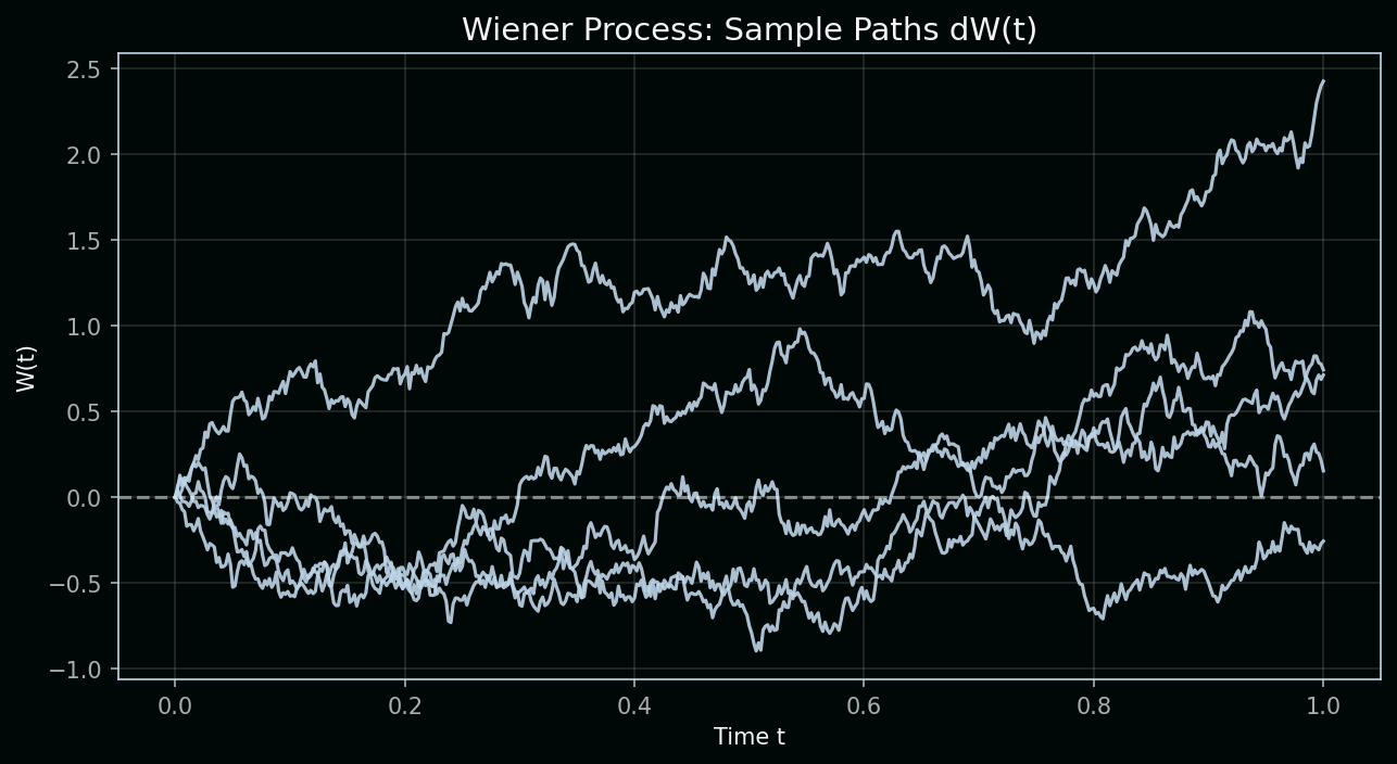
Reading the chart: The figure below shows five sample paths of a Wiener process W(t). Each path is one possible trajectory of pure random motion with no drift. Mathematically, we build W by summing independent increments dW—each drawn from a normal distribution with mean 0 and variance dt.

Variable	Definition	Role in the process
W(t)	Value of the Wiener process at time t	The cumulative sum of all random shocks; it can go up or down with no tendency to revert
dW	Increment of W over a small time step	dW ~ N(0, dt)—a random draw with variance proportional to the time step; smaller dt means smaller, finer shocks
t	Time	The horizontal axis; as t increases, W accumulates more randomness, so paths spread out

Key concept: The Wiener process has independent increments—the change from t₁ to t₂ is independent of the path before t₁. It also has zero drift and variance proportional to time: Var(W(t)) = t. That scaling is why we use √t when we talk about how far prices typically move over a horizon.

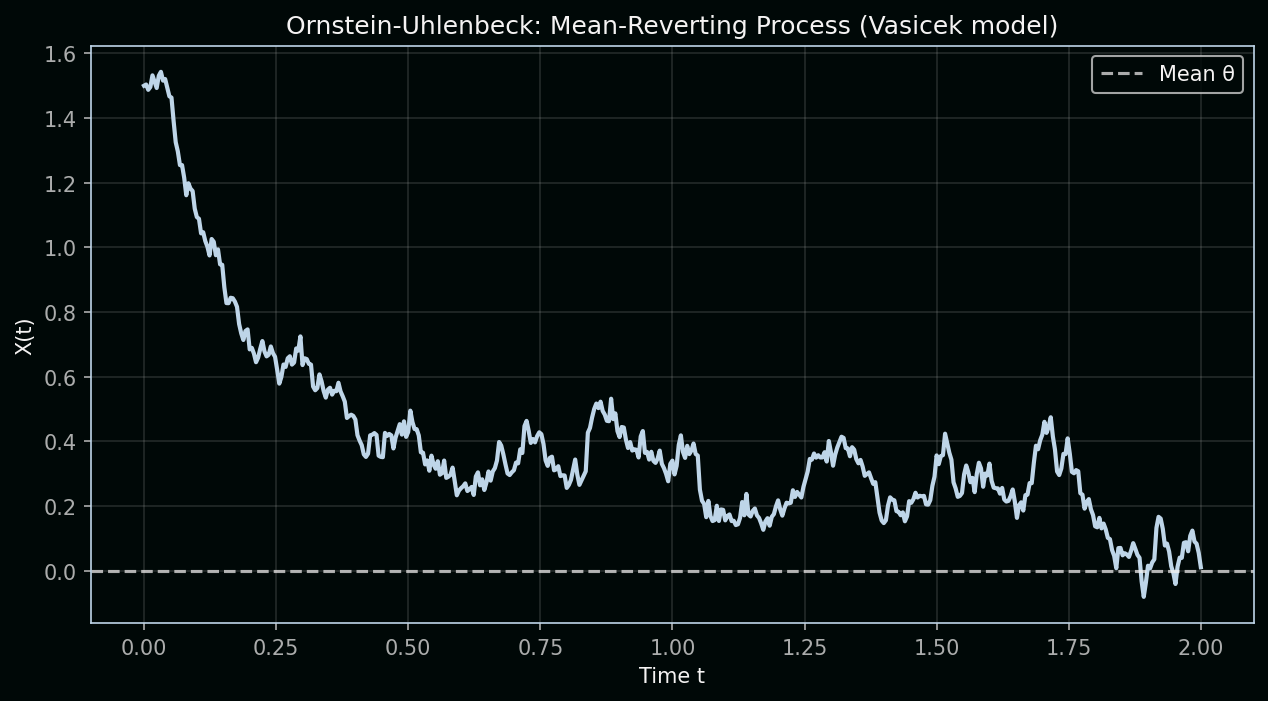
Ornstein–Uhlenbeck (1930): Mean Reversion

Ornstein and Uhlenbeck (1930) added friction: they modelled the velocity of a Brownian particle under drag. The result is a mean-reverting process—the farther you drift, the stronger the pull back. In finance, this became the Vasicek model for interest rates: prices don’t wander forever; they revert to a long-run level. That’s a crucial tweak to pure random walk.

The Ornstein-Uhlenbeck SDE:

dX = θ(μ − X)dt + σ dW

Variable	Definition	Role in the equation
X(t)	Current value of the process	What we observe (e.g., interest rate or spread); it evolves over time
θ	Mean-reversion speed	How quickly X is pulled back toward μ; larger θ = stronger pull, faster reversion
μ	Long-run mean	The level X tends to revert to; the “center of gravity” of the process
σ	Volatility	Size of the random shocks; scales the dW term so that diffusion remains significant
dW	Wiener increment	Same as before—random noise that perturbs X away from its mean

Key concept: The term θ(μ − X)dt is the mean-reverting drift. When X > μ, the drift is negative and pulls X down; when X < μ, the drift is positive and pulls X up. Unlike the Wiener process, X doesn’t wander off to infinity—it oscillates around μ. That’s why interest rates and some spreads are often modeled with OU: they tend to stay within a band.

---

In your Python stack, this “noise” is what we try to filter or model using TensorFlow and Keras. We treat asset prices as stochastic processes—often built on top of Brownian motion or its relatives.

---

2. 1900–1990s: Closed-Form Math, Then the Cracks Appear

For a long time, quants were “Formula Hunters.” Here’s the arc—and where it broke.

Bachelier → Black-Scholes: The Gaussian Era

• Bachelier (1900): First to treat stock prices as a random walk; first options formula.

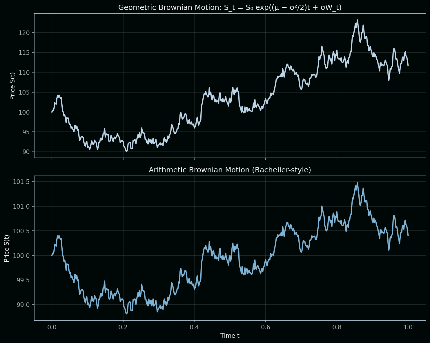
• Black–Scholes (1973): Assumed Geometric Brownian Motion (GBM):

  dS = μS dt + σS dW

  where S is the asset price, μ is drift, σ is volatility, and dW is a Wiener increment. Under GBM, log returns are normal. The analytic solution is:

  S_t = S₀ exp((μ − σ²/2)t + σW_t)

  The σ²/2 term comes from Itô’s lemma—quadratic variation of Brownian motion. Black and Scholes used this to derive their famous PDE and options formula. Today you can price a European option in SciPy or NumPy in two lines.

Variable definitions (GBM):

Variable	Definition	Role in the equation
S	Asset price at time t	What we are modeling; it evolves randomly but stays positive (multiply by S keeps it geometric)
μ	Expected return (drift)	Average growth rate; μS dt is the deterministic trend
σ	Volatility	Size of random fluctuations; σS dW scales noise with price (percent returns, not dollar)
dW	Wiener increment	Same pure randomness as before
S₀	Initial price	Starting value at t = 0
W_t	Cumulative Wiener process	Sum of all dW up to time t

Key concept (Itô correction): In ordinary calculus, d(exp(X)) = exp(X) dX. For Brownian motion, Itô’s lemma adds an extra term because W has quadratic variation—its “squared increments” accumulate. That’s why the exponent has (μ − σ²/2) instead of μ: the σ²/2 corrects for the convexity of the exponential. Without it, the expected value of S_t would be wrong.

Chart note: The top panel shows Geometric BM (Black-Scholes)—returns are multiplicative, prices stay positive. The bottom shows Arithmetic BM (Bachelier-style)—price changes add directly; prices can go negative. GBM is the standard for stocks.

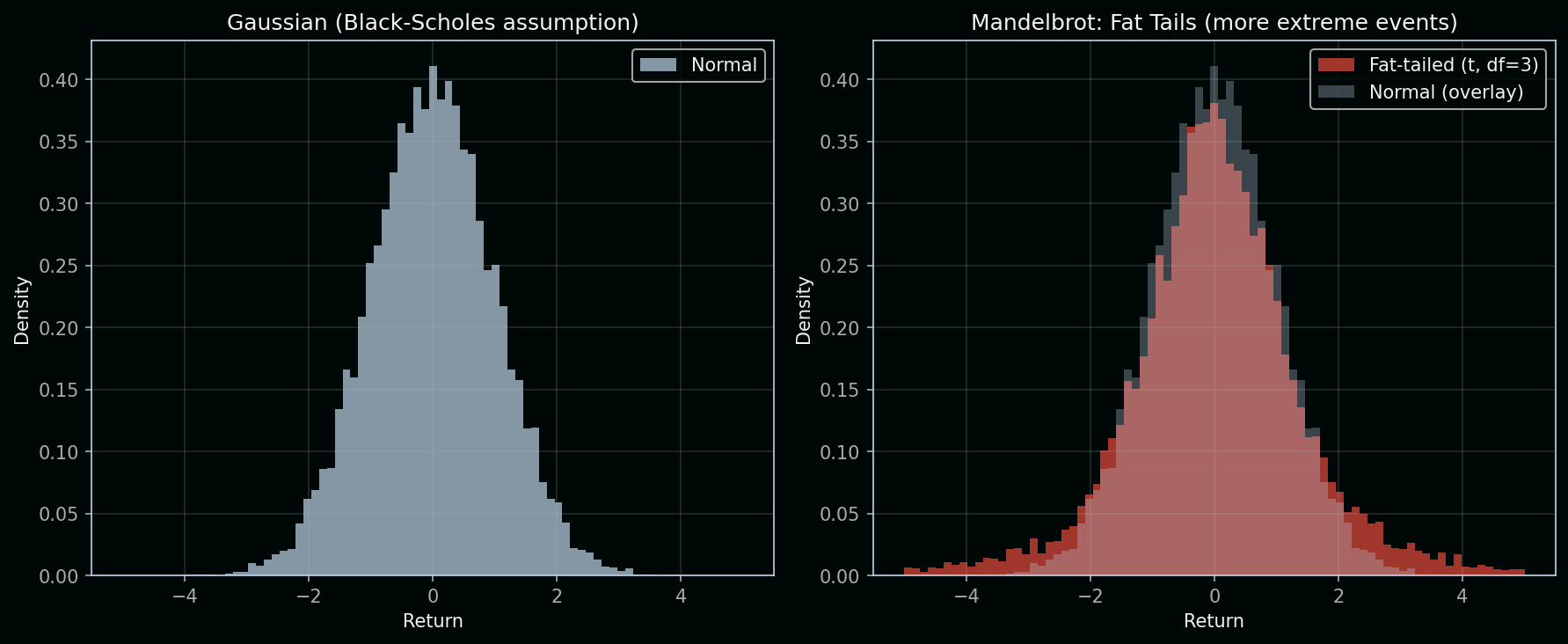
Mandelbrot (1963): The First Big Challenge

Benoit Mandelbrot analyzed cotton prices and showed that returns had fat tails—extreme moves happened far more often than a Gaussian predicts. He proposed stable Paretian (L-stable) distributions with infinite variance instead of the normal distribution. His student Eugene Fama confirmed this on Dow-Jones stocks: “no exceptions to the long-tailed nature of the distributions.” The idea was largely ignored by practitioners for decades—until crashes forced a reckoning.

Reading the chart: The left panel shows a Gaussian (normal) distribution—Black-Scholes’ assumption. Most returns cluster near zero; extreme events (|return| > 3) are rare. The right panel overlays a fat-tailed distribution (Student-t with 3 degrees of freedom): same center, but much more mass in the tails.

Variable	Definition	Role in the chart
Return	Log return or percentage change in price	The horizontal axis; we’re modeling its distribution
Density	Probability density at each return level	The vertical axis; height = how likely that return is
df (degrees of freedom)	Parameter of the Student-t	Lower df = fatter tails; df → ∞ gives the normal

Key concept: A fat-tailed distribution has more probability in the extremes than a Gaussian. Events like −5σ or +5σ are thousands of times more likely under fat tails. That’s why Black Monday, the 2008 crisis, and flash crashes are “impossible” under Black-Scholes but routine in reality—the tails matter for risk. Mandelbrot used stable distributions, which can have infinite variance; the Student-t is a tractable approximation with similar tail behavior.

1987 Black Monday: The Volatility Smile

On October 19, 1987, markets fell 20–25% in a day. After that, a persistent pattern appeared: the volatility smile. Out-of-the-money puts became systematically more expensive than Black-Scholes predicted. The model assumes constant volatility and log-normal returns; reality has time-varying volatility and fat tails. The smile proved that one size does not fit all strikes and maturities.

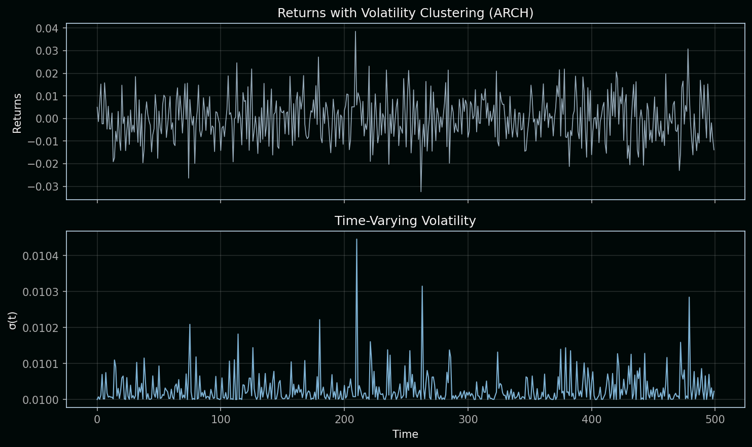
1982–1990s: ARCH and GARCH

Robert Engle introduced ARCH (1982) and Tim Bollerslev extended it to GARCH (1986). These models capture what simple Brownian motion cannot:

• Volatility clustering: Big moves tend to follow big moves.
• Time-varying variance: Vol is not constant.
• Fat-tailed unconditional distributions.

By the 1990s, ARCH/GARCH were standard in risk and econometrics. They formalized Mandelbrot’s intuition: volatility is predictable in structure, even if levels are not.

Reading the chart: The top panel shows returns over time. Notice how large moves tend to cluster—bursts of high volatility followed by quieter periods. The bottom panel shows σ(t), the time-varying volatility driving those returns. It spikes when returns are large and decays when they’re small.

ARCH(1) specification:

r_t = σ_t · ε_t,    where ε_t ~ N(0,1)
σ²_{t+1} = ω + α · r_t²

Variable	Definition	Role in the equation
r_t	Return at time t	Observable; we model it as volatility × a standard normal shock
σ_t	Conditional volatility at time t	Unobserved; it scales the random shock so that variance changes over time
ε_t	Standard normal innovation	ε_t ~ N(0,1); the “unit” randomness, same for all t
ω	Base variance (constant)	Floor for σ²; ensures volatility doesn’t collapse to zero
α	Persistence of squared returns	How much today’s squared return feeds into tomorrow’s volatility; α > 0 creates clustering

Key concept: Volatility clustering means big moves beget big moves. When r_t is large, r_t² is large, so σ²_{t+1} rises—the next period has higher volatility. When returns are small, σ² drifts back down. This is exactly what GBM cannot do: in Black-Scholes, volatility is constant. ARCH/GARCH let volatility be a function of past returns, matching the “burstiness” we see in real markets.

---

The takeaway: Formulas assume the world is Gaussian. Mandelbrot, Black Monday, and ARCH/GARCH showed it isn’t. That’s where machine learning and data-driven models enter—to capture patterns that closed-form math cannot.

3. The Shift to “Data-First” Quant Dev

In the last decade, the “Quant Dev” role evolved. We moved from solving equations to Training Models.

Era	Focus	Primary Tool
1980s	Derivatives Math	Pen & Paper / Fortran
2000s	Speed & Execution	C++ / Java
2025+	Alpha & LLMs	Python / TensorFlow / PyTorch

4. Why LLMs in Quant Dev?

You mentioned using LLMs. This is the bleeding edge.

• Sentiment Analysis: Using an LLM to “read” 10,000 news articles in a second to see if the market is scared.
• Feature Engineering: Using AI to find hidden correlations between “Weather in Brazil” and “Coffee Future Prices” that a human would never see.

---

Our Tech Stack Roadmap

Since we are focusing on the Python ecosystem, our journey will look like this:

1. Data Wrangling: Mastering Pandas and NumPy for massive financial datasets.
2. Visualization: Using Matplotlib and Plotly to see the “signal” in the “noise.”
3. Deep Learning: Building Predictors with Keras and TensorFlow.
4. LLM Integration: Using LangChain or OpenAI/Local LLMs to process unstructured financial data.

Accuracy Note: While we use Python for its incredible ML libraries, remember that Python is “slow” compared to C++. As a Quant Dev, you will learn to use Vectorization (NumPy) to make Python run at near-C speeds.

---

Summary: Quant Dev Then and Now

Quantitative development has shifted from pen-and-paper math to Python-based machine learning and LLM-powered analysis. The core idea—finding signal in market noise—remains; the tools are now Pandas, TensorFlow, and large language models. If you’re starting a quant dev career today, focus on data wrangling, visualization, deep learning, and LLM integration. The formulas matter for context, but the alpha comes from data and models.

---

Tags: #QuantDev #Python #MachineLearning #TensorFlow #BrownianMotion #Mandelbrot #ARCH #GARCH #VolatilitySmile #FinancialHistory #AlgorithmicTrading #QuantitativeFinance

Back to all posts